Expectation Maximization (EM)
EM is an algorithm for finding the maximum likelihood parameters $\theta$ for probabilistic models having latent variables. EM consists of two steps E (Expectation) and M (Maximization). EM is a special case of a MM algorithm for optimization.
Suppose we want to find the maximum likelihood for a probabilistic model with latent variables. The set of observed variables is given by $\mathbf{x}$ while the set of latent variables is given by $\mathbf{z}$. Suppose the joint distribution is parameterized by $\theta$, $p(\mathbf{x}, \mathbf{z}|\theta)$. Suppose we need to maximize the likelihood of the observed data; therefore, we seek find the parameters $\theta$ that maximize the likelihood of the marginal distribution $p(\mathbf{x}|\theta)$. Although optional, it is common practice to use the log-likelihood. The log likelihood function of the observed variables is given by
\[\log p(\mathbf{x}|\theta) = \log \sum_{\mathbf{z}} p(\mathbf{x}, \mathbf{z}|\theta)\]The underlying assumption is that $p(\mathbf{x},\mathbf{z}|\theta)$ yields an easier optimization problem then $p(\mathbf{x}|\theta)$. For any choice of distribution $q$ over $\mathbf{z}$, the following holds:
\[\log p(\mathbf{x}|\theta) = \mathcal{L}(q,\theta) + \text{KL}(q||p)\]where
\[\mathcal{L}(q, \theta) = \sum_{\mathbf{z}} q(\mathbf{z}) \log \frac{p(\mathbf{x},\mathbf{z}|\theta)}{q(\mathbf{z})}\] \[\text{KL}(q||p) = -\sum_{\mathbf{z}} q(\mathbf{z}) \log \frac{p(\mathbf{z}|\mathbf{x},\theta)}{q(\mathbf{z})}\]Proof
$$ \mathcal{L}(q, \theta) = \sum_{\mathbf{z}} q(\mathbf{z}) [\log p(\mathbf{x},\mathbf{z}|\theta) - \log q(\mathbf{z})]$$ $$ \mathcal{L}(q, \theta) = \sum_{\mathbf{z}} q(\mathbf{z}) [\log p(\mathbf{z}|\mathbf{x},\theta) + \log p(\mathbf{x}) - \log q(\mathbf{z})]$$ $$ \mathcal{L}(q, \theta) = \sum_{\mathbf{z}} q(\mathbf{z}) [\log p(\mathbf{z}|\mathbf{x},\theta) - \log q(\mathbf{z})] + \log p(\mathbf{x}) $$ $$ \mathcal{L}(q, \theta) = -\text{KL}(q||p) + \log p(\mathbf{x}) $$Since $\text{KL}(q||p) \ge 0$, then it follows that $\mathcal{L}(q,\theta) \le \log p(\mathbf{x})$. Therefore $\mathcal{L}(q,\theta)$ is a lower bound to $\log p(\mathbf{x})$.
Suppose the current parameters are denoted by $\theta^{\text{old}}$. In E-step, the lower bound $\mathcal{L}(q,\theta^\text{old})$ is maximized with respect to $q$ with $\theta^\text{old}$ fixed. The tightest lower bound $\mathcal{L}(q,\theta^\text{old})$ occurs when $q(\mathbf{z}) = p(\mathbf{z}|\mathbf{x},\theta^\text{old})$ since the KL divergence term disappears and as a result, $\mathcal{L}(q,\theta^\text{old}) = \log p(\mathbf{x} | \theta^{\text{old}})$. Note for $q(\mathbf{z}) = p(\mathbf{z}|\mathbf{x},\theta^\text{old})$, $\mathcal{L}(q, \theta) \le \log p(\mathbf{x}| \theta)$ for $\theta \neq \theta^{\text{old}}$ but achieves equality for $\theta = \theta^\text{old}$. $\mathcal{L}(p(\mathbf{z}|\mathbf{x},\theta^\text{old}), \theta)$ can be seen as a minorizing surrogate function for $\log p(\mathbf{x}|\theta)$.
In the M-step, the distribution $q(\mathbf{z}) = p(\mathbf{z}|\mathbf{x},\theta^\text{old})$ is held fixed but the lower bound is maximized with respect to the parameters $\theta$. The updated parameters are denoted by $\theta^\text{new}$. Recall that $\mathcal{L}(q, \theta^{\text{old}}) = \log p(\mathbf{x} | \theta^{\text{old}})$, $\log p(\mathbf{x} | \theta^{\text{old}}) \le \mathcal{L}(q, \theta^\text{new})$. Since $q(\mathbf{z}) = p(\mathbf{z}|\mathbf{x},\theta^\text{old})$, $\mathcal{L}(q, \theta^\text{new}) \le \log p(\mathbf{x}|\theta^\text{new})$ and therefore $\log p(\mathbf{x} | \theta^{\text{old}}) \le \log p(\mathbf{x} | \theta^{\text{new}})$. In next E-step, $q(\mathbf{z})$ will be set to $p(\mathbf{z}|\mathbf{x},\theta^\text{new})$ thus re-establishing equality, and in the following M-step, the new parameters will increase or maintain the same likelihood.
In the E-step, if we set $q(\mathbf{z}) = p(\mathbf{z}|\mathbf{x},\theta^\text{old})$
\[\mathcal{L}(q, \theta) = \sum_{\mathbf{z}}p(\mathbf{z}|\mathbf{x},\theta^\text{old}) \log \frac{p(\mathbf{x},\mathbf{z}|\theta)}{p(\mathbf{z}|\mathbf{x},\theta^\text{old})}\] \[\mathcal{L}(q, \theta) = \sum_{\mathbf{z}}p(\mathbf{z}|\mathbf{x},\theta^\text{old}) [\log p(\mathbf{x},\mathbf{z}|\theta) - \log p(\mathbf{z}|\mathbf{x},\theta^\text{old})]\]Since the second term does not rely on $\theta$ during the M-step it is considered a constant and as a result, the M-step effectively optimizes $Q$:
\[\mathcal{L}(q, \theta) = \sum_{\mathbf{z}}p(\mathbf{z}|\mathbf{x},\theta^\text{old}) \log p(\mathbf{x},\mathbf{z}|\theta) + \text {constant}\] \[Q(\theta, \theta^{\text{old}}) = \sum_{\mathbf{z}}p(\mathbf{z}|\mathbf{x},\theta^\text{old}) \log p(\mathbf{x},\mathbf{z}|\theta) = \mathbb{E}_{p(\mathbf{z}|\mathbf{x},\theta^\text{old})}[\log p(\mathbf{x},\mathbf{z}|\theta) ]\]The quantity in the expectation is the log likelihood of the complete distribution, and in order to evaluate $Q$ we need to evaluate $p(\mathbf{z}|\mathbf{x},\theta^\text{old})$. Typically the primary focus of the E-step is to evaluate $p(\mathbf{z}|\mathbf{x},\theta^\text{old})$.
EM Algorithm:
-
Initialize $\theta^{\text{old}}$
-
E-Step: Evaluate $p(\mathbf{z}|\mathbf{x},\theta^\text{old})$.
-
M-Step: $\theta^{\text{new}} = \text{argmax}_\theta Q(\theta, \theta^{\text{old}})$
-
If not converged, $\theta^{\text{old}} \gets \theta^{\text{new}}$ and go to step 2.
Toy Example
Our dataset is generated using the following Gaussian mixture:
\[p(x|\mu) = \frac{1}{2} \mathcal{N}(x|2, 1) + \frac{1}{2} \mathcal{N}(x|-2,1)\]and consists of $1000$ samples.
Suppose we have a Gaussian Mixture that is parameterized as such
\[p(x|\mu) = \frac{1}{2} \mathcal{N}(x|\mu, 1) + \frac{1}{2} \mathcal{N}(x|-\mu, 1)\]We will add a binary random variable $z \in {0,1}$ with probability $1/2$ that will act like our latent variable that incidates “membership” to a particular Gaussian $\mathcal{N}(x|\mu, 1)$ or $\mathcal{N}(x|-\mu, 1)$. The joint distribution of $x,z$ is as follows
\[p(x,z|\mu) = \frac{1}{2}^{z}\mathcal{N}(x| \mu,1)^{z}\frac{1}{2}^{1-z}\mathcal{N}(x| -\mu,1)^{1-z}\]Note $p(x) = \sum_{z \in {0,1}} p(x, z)$ recovers the original marginal distribution.
In the E-step we need to evaluate posterior distribution $p(z | x;\mu_\text{old})$ at the old parameters
\[p(z | x;\mu) = \frac{p(x,z| \mu)}{p(x|\mu)}\] \[= \frac{\frac{1}{2}^{z}\mathcal{N}(x| \mu,1)^{z}\frac{1}{2}^{1-z}\mathcal{N}(x| -\mu,1)^{1-z}}{\frac{1}{2} \mathcal{N}(x|\mu, 1) + \frac{1}{2} \mathcal{N}(x|-\mu, 1)}\]Therefore
\[p(z = 1 | x;\mu) = \gamma_1(\mu) = \frac{\frac{1}{2}\mathcal{N}(x| \mu,1)}{\frac{1}{2} \mathcal{N}(x|\mu, 1) + \frac{1}{2} \mathcal{N}(x|-\mu, 1)}\] \[p(z = 0| x;\mu) = \gamma_0(\mu) = \frac{\frac{1}{2}\mathcal{N}(x| -\mu,1)}{\frac{1}{2} \mathcal{N}(x|\mu, 1) + \frac{1}{2} \mathcal{N}(x|-\mu, 1)}\]$\gamma$ is sometimes called the responsibilities.
In the M-step, we need to maximize $Q(\mu, \mu_\text{old}) = \mathbb{E}_{p(z|x,\mu^\text{old})}[\log p(\mathbf{x},\mathbf{z}|\mu) ]$
\[Q(\mu, \mu_\text{old}) = \sum_{z \in {0,1}} \gamma_z(\mu_\text{old}) \log p(x,z|\mu)\] \[Q(\mu, \mu_\text{old}) = \gamma_1(\mu_\text{old})[\log \frac{1}{2} + \log \mathcal{N(x|\mu)}] + \gamma_0(\mu_\text{old})[\log \frac{1}{2} + \log \mathcal{N(x|-\mu)}]\]The optimal $\mu^\star$ satisfies
\[\frac{d}{d\mu}Q(\mu,\mu_\text{old})\bigg|_{\mu = \mu_\text{new}} = 0\]Using [2], the derivative is:
\[\frac{d}{d\mu}Q(\mu,\mu_\text{old}) = \gamma_1(\mu_\text{old})(x-\mu) - \gamma_0(\mu_\text{old})(x+\mu)\] \[\mu_\text{new}= (\gamma_1(\mu_\text{old}) - \gamma_0(\mu_\text{old})) x\]Since the data is assumed to be sampled the i.i.d for a dataset, the update rule is
\[\mu_\text{new}= \frac{1}{N}\sum_{n = 1}^N (\gamma_1^{(n)}(\mu_\text{old}) - \gamma^{(n)}_0(\mu_\text{old})) x_i\]This is result of the decomposability of $Q$ under iid conditions. Set $Z={z_1,…,z_N}$ and $X = {x_1, …, x_N}$
\[\mathbb{E}_{p(Z|X,\mu^\text{old})}[\log p(X, Z|\mu) ] = \mathbb{E}_{p(Z|X,\mu^\text{old})}[\sum_n \log p(x_n, z_n|\mu) ]\]by linearity of expectation,
\[\sum_n \mathbb{E}_{p(Z|X,\mu^\text{old})}[\log p(x_n, z_n|\mu) ]\]by the i.i.d assumption
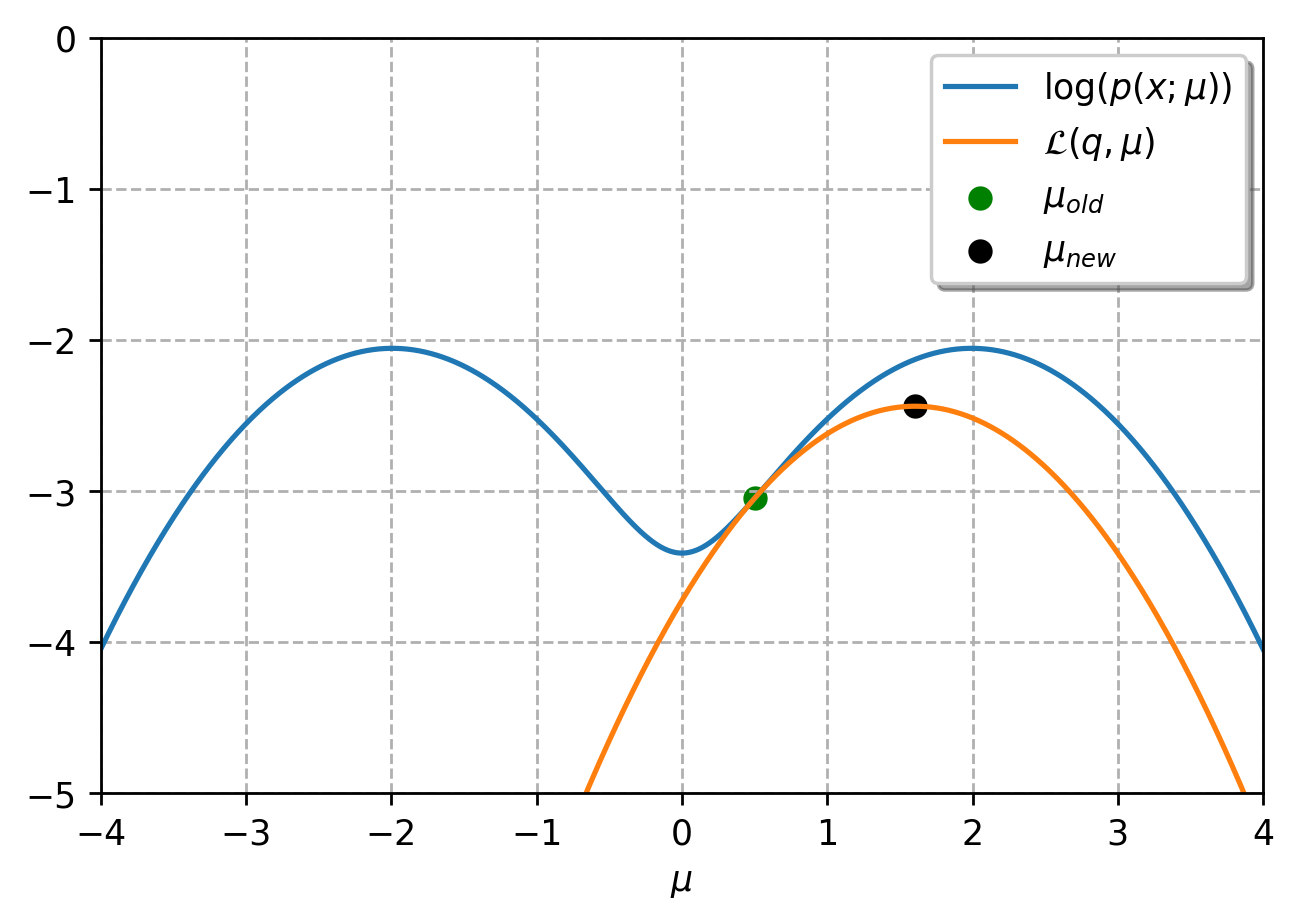
\[\sum_n \mathbb{E}_{p(z_n|x_n,\mu^\text{old})}[\log p(x_n, z_n|\mu) ]\]We initialize $\mu_\text{old} = .5$ and run the EM algorithm:


Note that the lower bound achieves equality with the log marginal likelihood at $\mu_\text{old}$ and it is concave unlike the log marginal likelihood.
Also, note that initializing at $\mu = 0$ causes the responsibilities cancel out for all $x_n$, therefore the next $\mu_\text{new}$ will be zero. This example shows that EM doesn’t necessarily converge to local maxima, and it can get stuck in stationary points.
References
[1] Bishop, Christopher M. Pattern Recognition and Machine Learning. Springer, 2006.
[2] Petersen, Kaare Brandt, and Michael Syskind Pedersen. “The matrix cookbook.” Technical University of Denmark 7.15 (2008): 510.
[3] Sun, Ying, Prabhu Babu, and Daniel P. Palomar. “Majorization-minimization algorithms in signal processing, communications, and machine learning.” IEEE Transactions on Signal Processing 65.3 (2016): 794-816.