Neural Ordinary Differential Equations
Ordinary Differential Equations (ODEs)
Solving an ODE consists finding of the $h(t)$ that satisfies:
\[\frac{d}{dt}h(t) = f(t, h(t)) \quad 0 \leq t \leq T\] \[h(0) = h_0\]where $h_0$ is the initial condition. General ODEs are often impossible to solve for generic $f$, and they generally require numerical methods in order to provide a solution.
Numerical Solutions to ODEs
Euler’s Method
Solving the ODE:
\[\frac{d}{dt}h(t) = f(t, h(t)) \quad 0 \leq t \leq T\] \[h(0) = h_0\]Suppose we will need to evaluate the solution $h(t)$ at fixed increments: \(0 = t_0 < t_1 < ... < t_{N-1} < t_N = T\)
The step size is given by:
\[\Delta t= T/N\]Euler’s method provides an algorithm for estimating the solution at fixed time steps.
Developing Euler’s Method
Suppose $h(t)$ is the solution to the ODE above and we expand $h(t)$ using a Taylor series about $t=t_i$:
\[h(t) = h(t_i) + h'(t_i)(t - t_i) + \frac{1}{2}(t- t_i)^2 h''(\xi)\]where $t_i \in [0,T]$ and $\xi \in [t, t_i]$
If we evaluate $t=t_{i+1}$, define $\Delta t = t_{i+1} - t_i$, and substitute $h'(t_i) = f(t_i, h(t_i))$:
\[h(t_{i+1}) = h(t_i) + f(t_i, h(t_i)) \Delta t + \frac{1}{2} \Delta t^2 h''(\xi)\]Dropping the error term $\frac{1}{2} \Delta^2 h''(\xi)$ provides Euler’s method:
\[h(t_{i+1}) = h(t_i) + f(t_i, h(t_i)) \Delta t\]We denote $h(t_{i}) = h_{t_{i}}$, Euler’s method is rewritten as:
\[h_{t_{i+1}} = h_{t_{i}} + f(t_i, h_{t_{i}}) \Delta t\]Euler’s Method from a Riemman Sum
From the fundamental theorem of calculus:
\[h(t_{i+1}) - h(t_i) = \int_{t_{i+1}}^{t_i} f(t, h(t)) dt\]The right hand integral can be approximated using left-hand Riemman sum:
\[\int_{t_{i+1}}^{t_i} f(t, h(t)) dt \approx f(t_i,h) \Delta t\] \[h(t_{i+1}) = h(t_i) + \int_{t_{i+1}}^{t_i} f(t, h(t)) dt\] \[h(t_{i+1}) = h(t_i) + f(t_i,h(t_i)) \Delta t\]Taylor Methods
If the higher order derivatives of $f$ are accessible, that information can be incorporated in order to enhance Euler’s method. A second order Taylor method has following update:
\[h_{t_{i+1}} = h_{t_{i}} + \Delta t f(t_{i}, h_{t_{i}}) + \frac{\Delta t^2}{2} \frac{d}{dt} f(t_{i}, h_{t_{i}})\]Other ODE Solvers
Most ODE solvers build on Euler’s method. Different solvers have varying pros and cons in terms of approximation error, evaluation speed, and stability.
Runge–Kutta Methods
The second-order Runge-Kutta method (RK2):
\[h_{t_{i+1}} = h_{t_i} + \frac{\Delta t}{4}(f(t_i, h_{t_i}) + 3 f(t_i + \frac{2}{3}\Delta t, \bar{h}))\]where
\[\bar{h} = h_{t_i} + \frac{2}{3} \Delta t f(t_i, h_{t_i})\]The classical fourth-order Runge-Kutta method (RK4) is defined as follow:
\[h(t_{i+1}) = h(t_i) + \frac{1}{6}(k_1 + 2k_2 + 2k_3 + k_4)\]where
\[k_1 = \Delta t f(t_i, h_{t_i})\] \[k_2 = \Delta t f(t_i + \frac{\Delta t}{2}, h_{t_i}+ \frac{k_1}{2})\] \[k_3 = \Delta t f(t_i + \frac{\Delta t}{2}, h_{t_i}+ \frac{k_2}{2})\] \[k_4 = \Delta t f(t_i+\Delta t, h_{t_i} + k_3)\]ResNets and ODEs
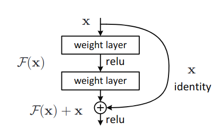
ResNet are a particular class of neural network models that enable the training of models with hundreds of layers. The underlying principle of ResNet is the idea of residual learning. Suppose $\mathcal{H}(x)$ is a desired mapping at specific layer, and in residual learning, we let the previous stacked non-linear layers a different mapping $\mathcal{F}(x) = \mathcal{H}(x) - x$. The original problem of learning of $\mathcal{H}(x)$ is recast as learning the following $\mathcal{F}(x) + x$. $\mathcal{F}(x)$ called the residual mapping. The residual mapping contains the trainable parameters for its layer so the residual mapping $\mathcal{F}(x;\theta_\ell)$, where $\theta_\ell$ are the trainable parameters at layer $\ell$. The underlying assumption of residual learning is that it is simpler to learn the residual mapping $\mathcal{F}(x)$ relative to the target mapping $\mathcal{H}(x)$.

The residual mapping echoes Euler’s method. If we set $h_\ell = x$, $F(h_\ell,\theta_\ell) = \mathcal{F}(x, \theta)$, and $h_{\ell+1} = \mathcal{H}(x, \theta)$:
\[h_{\ell+1} = h_\ell + F(h_\ell, \theta_\ell)\]If $F(h_\ell, \theta_\ell) = \Delta t f(h_\ell, \theta_\ell)$, where $\Delta t > 0$
\[h_{\ell+1} = h_\ell + \Delta t f(h_\ell, \theta_\ell)\]Here the index $\ell$ indicates the $\ell^{\text{th}}$ layer in the ResNet network and $\Delta t > 0$ is the step size. In the limit of adding more layers and taking a smaller size,
\[\frac{d}{dt} h(t) = f(t, h(t),\theta)\]The initial condition condition $h(0)=h_0$ is the input layer and the output layer is the value at $h(T) = h_T$ [4]. In this sense, the network can be seen as having continuous depth. The output value $h(T)$ can be evaluated using a blackbox differential equation to a desired accuracy.
Backpropagating Through ODE Solutions
In order to train a continuous-depth network, one needs to backpropagated through an ODE solver. Unrolling the solver and backpropagating through the operations incurs a high memory cost and an additional numerical error. Instead the approach presented in [1] treats the ODE solver as a blackbox and computes the gradient using a method called adjoint sensitivity method.
Consider minimizing the following loss function $\mathcal{L}$:
\[\mathcal{L}(z(t_{i+1})) = \mathcal{L}\bigg(z(t_i) + \int_{t_i}^{t_{i+1}} f(z(t),t,\theta) dt \bigg) = \mathcal{L}(\text{ODESolve}(z(t_i),f,t_i,t_{i+1},\theta))\]where $z(t)$ is a hidden state function that follows $\frac{d}{dt} z(t) = f(z(t), t, \theta)$ where $\theta$ are the parameters. Evaluating the gradient $\frac{\partial \mathcal{L}}{\partial z(t)}$ is necessary in order to compute the gradient of $\mathcal{L}$ with respect to the parameters $\theta$. The gradient $\frac{\partial \mathcal{L}}{\partial z(t)}$ is called the adjoint state $a(t)$. The dynamics of the adjoint are given by the following ODE:
\[\frac{d}{dt} a(t) = -a(t)^\text{T} \frac{\partial f(z(t), t, \theta)}{\partial z(t)}\]In order to compute $\partial \mathcal{L} /\partial \mathbf{z}(t_0)$, the value of $a(t_0)$ needs to be determined which is the solution to the following ODE:
\[a(t_0) = a(t_1) + \int_{t_1}^{t_0} -a(t)^\text{T} \frac{\partial f(z(t), t, \theta)}{\partial z(t)} dt\]where $a(t_1) = \partial \mathcal{L} /\partial \mathbf{z}(t_1)$. Therefore, the ODE solver needs to run backwards with $\partial \mathcal{L} /\partial \mathbf{z}(t_1)$ as the initial condition. In order to solve for $a(t)$, the ODE solver needs access to $z(t)$, and another observation is that the values of $\frac{\partial \mathcal{L}}{\partial z(t)}$ need to be computed in a backwards manner similar to backpropagation. Also, the $\frac{\partial \mathcal{L}}{\partial z(t_N)}$ is simply the gradient of cost function computed with respect to the last time step, and it serves as the initial condition for the whole backwards computation.
Proof of $\frac{d}{dt} a(t) = -a(t)^\text{T} \frac{\partial f(z(t), t, \theta)}{\partial z(t)}$
For simplicity, we assume $z$ and $f$ are scalar functions.
If we treat $z(t)$ as hidden layers in a neural network. $z(t+\varepsilon)$ is the next hidden layer in the network. $z(t+\varepsilon)$ and $z(t)$ are related by the following relationship:
\[z(t+\varepsilon) = z(t) + \int_{t}^{t+\varepsilon} f(z(t), t, \theta) dt = T_{\varepsilon}(z(t), t)\]Similarly, $T_{\varepsilon}(z(t), t)$ can be approximated using a Taylor series at $t$:
\[z(t+\varepsilon) = z(t) + f(z(t), t, \theta) \varepsilon + \frac{1}{2} \frac{d}{dt}f(z(t), t, \theta)\big|_{t = \xi \in [t, t+\varepsilon]} \varepsilon^2\] \[z(t+\varepsilon) = z(t) + f(z(t), t, \theta) \varepsilon + O(\varepsilon^2)\]By chain rule, the gradient between the two layers by the following:
\[\frac{\partial \mathcal{L}}{\partial z(t)} = \frac{\partial \mathcal{L}}{\partial z(t+\varepsilon)} \frac{\partial z(t+\varepsilon)}{\partial z(t)}\]Using $a(t) = \partial \mathcal{L} / \partial z(t)$
\[a(t) = a(t+\varepsilon) \frac{\partial T_\varepsilon(z(t), t)}{\partial z(t)}\]Using the definition of the derivative:
\[\frac{d a(t)}{dt} = \text{lim}_{\varepsilon \rightarrow 0} \frac{a(t+\varepsilon) - a(t)}{\varepsilon}\] \[\text{lim}_{\varepsilon \rightarrow 0} \frac{a(t+\varepsilon) - a(t+\varepsilon)\frac{\partial }{\partial z(t)}\left( z(t) + \varepsilon f(z(t), t, \theta) + O(\varepsilon^2) \right)}{\varepsilon}\] \[\text{lim}_{\varepsilon \rightarrow 0} -a(t+\varepsilon)\frac{\partial}{\partial z(t)}f(z(t), t, \theta) + O(\varepsilon)\] \[=-a(t)\frac{\partial}{\partial z(t)}f(z(t), t, \theta)\]To compute $\frac{\partial}{\partial \theta} \mathcal{L}$, the following integral needs to be evaluated:
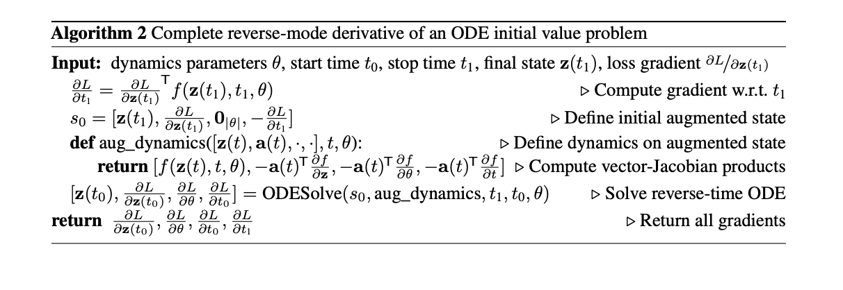
\[\frac{\partial}{\partial \theta} \mathcal{L} = - \int_{t_1}^{t_0} a(t)^T \frac{\partial f(z(t), t, \theta)}{\partial \theta} dt\]$a(t)$ and $z(t)$ need to be computed before $\frac{\partial}{\partial \theta} \mathcal{L}$ can be computed. $a(t)$ and $\frac{\partial}{\partial \theta} \mathcal{L}$ can be evaluted using an ODE solver on an augumented ODE.
Building the Augumented ODE
Since $\frac{\partial}{\partial t}\theta(t) = \mathbf{0}$ and $\frac{d}{dt} t(t) = 1$
\[\frac{d}{dt} \begin{bmatrix} z \\ \theta \\ t \end{bmatrix} = \begin{bmatrix} f(z(t), t, \theta) \\ 0 \\ 1 \end{bmatrix} = f_{\text{aug}}(z, \theta, t)\] \[a_{\text{aug}} = \begin{bmatrix} a \\ a_\theta \\ a_t \end{bmatrix} \text { where } a_{\theta}(t) = \frac{dL}{d\theta(t)}, a_t(t) = \frac{dL}{dt(t)}, a(t) = \frac{\partial \mathcal{L}}{\partial z(t)}\]The Jacobian $f_{\text{aug}}(z, \theta, t)$ w.r.t to $z, t, \theta$ is
\[\frac{\partial}{\partial [z, t, \theta]} f_{\text{aug}}(z, \theta, t) = \begin{bmatrix} \frac{\partial}{\partial z}f & \frac{\partial}{\partial t}f & \frac{\partial}{\partial \theta} f \\ 0 & 0 & 0\\ 0 & 0 & 0 \end{bmatrix}\] \[\frac{d}{dt} a_\text{aug}(t) = -\begin{bmatrix} a(t)^T & a_\theta(t)^T & a_t(t)^T\end{bmatrix} \frac{\partial}{\partial [z, t, \theta]} f_{\text{aug}}(z, \theta, t) = -\begin{bmatrix} a(t)^T \frac{\partial}{\partial z}f & a(t)^T \frac{\partial}{\partial \theta}f & a(t)^T \frac{\partial}{\partial t}f \end{bmatrix}\]From the equation above and setting $a_\theta(t_N) = 0$,
\[a_\theta(t_0) = \frac{\partial}{\partial \theta} \mathcal{L} = -\int_{t_N}^{t_0} a(t)^T \frac{\partial}{\partial \theta} f(z(t), \theta, t) dt\]The gradients w.r.t $t_0$ and $t_N$ are given by
\[a_t(t_N) = \frac{\partial \mathcal{L}}{dt_N} = a(t_N) f(z(t_N), t_N ,\theta) = \frac{\partial \mathcal{L}}{\partial z(t_N)} f(z(t_N), t_N ,\theta)\] \[a_t(t_0) = \frac{\partial \mathcal{L}}{dt_0} = a_t(t_N) -\int_{t_N}^{t_0} a(t)^T \frac{\partial}{\partial \theta} f(z(t), \theta, t) dt\]Note how the gradient for $t_N$ needs to be computed before $t_0$, and $t_0$ is solved in a “backwards” manner.
The overall algorithm for backprop through the ODE solution is given by

TorchDiffEq and torchdyn both implement various neural ODE algorithms.
References:
- Chen, Tian Qi, et al. “Neural ordinary differential equations.” Advances in neural information processing systems. 2018.
- He, Kaiming, et al. “Deep residual learning for image recognition.” Proceedings of the IEEE conference on computer vision and pattern recognition. 2016.
- Bradie, B. (2006). A friendly introduction to numerical analysis. Upper Saddle River, NJ: Pearson Prentice Hall.
- Chang, Bo, et al. “Multi-level residual networks from dynamical systems view.” arXiv preprint arXiv:1710.10348 (2017).